Exploratory Data Analysis with R and DPLYR
Antonio Ruiz August 12, 2019
Who is this for ?
This quick little walk through is meant to highlight some of the power of Exploratory Data Analysis with R’s DPLYR package. It is assumed you have some basic programming knowledge of R. If you dont, no worries, there’s plenty of resources out there to help. https://www.datamentor.io/r-programming/operator/
What is Exploratory Data Analysis
Exploratory data analysis is arguably the most crucial step of any data science experiment. It is in this phase of the data science life cycle that the data is evaluated, variables are cataloged, and we can begin to come up with a strategy on how we want further analyze our dataset. Poor preliminary data analysis could spell trouble and unnecessary head aches down the road.
What is DPLYR
DPLYR is a R library that is meant to make your data cleansing experience feel natural and readable. DPLYR uses the “%>%” operator (called the pipe operator) to apply some sort of action or change to the dataset. With just a few short commands, we can create new variables, filter out unecesaary rows, and columns, and even transform our dataset. This is an introductory tutorial, so we are going to be focusing on the filter() and mutate() functions.
Libraries
We will be featuring the DPLYR library. For more information, click the following link. https://cran.r-project.org/web/packages/dplyr/vignettes/dplyr.html
##
## Attaching package: 'dplyr'

## The following objects are masked from 'package:stats':
##
##     filter, lag

## The following objects are masked from 'package:base':
##
##     intersect, setdiff, setequal, union
Loading Data
The read.table() function is used to read a tabular text file of data into a dataframe. One common mistake that many beginners make is trying to load data outside of their current working directory. A good habit of mine is to use to the setwd() command to tell R to where my I am going to be working out of.
# Set the working directory to my folder where my files will be located
setwd("C:/Users/tony/Desktop/workspace/ML/EDA")

# Syntax)
#   dataframe <- read.table("Filepath", header=True)
data <- read.table("hw03data.txt", header=TRUE)
Basic Exploratory Analysis
Gaining A Feel for the Data
The head() command is typically the first thing I go to when the data is loaded. If the data us properly loaded, you will be able to see the first five observations from your table. Similarly, you can use the tail() command to view the last five observations.
head(data)
##    id gender ageGroup pulse temp virus
## 1 101      F        2    58   97     N
## 2 102      M        2    55   98     N
## 3 103      F        0    51   97     N
## 4 104      M        1    68   98     Y
## 5 105      F        0    77   98     Y
## 6 106      M        0    56   97     N
You also are not limited to five observations, use the ‘n’ parameter within the function to change the number of observation shown.
tail(data, n = 10 )
##        id gender ageGroup pulse temp virus
## 4991 5091      F        0    59   97     N
## 4992 5092      F        2    64   97     N
## 4993 5093      F        2    57   98     N
## 4994 5094      M        2    54   97     N
## 4995 5095      M        2    44   99     N
## 4996 5096      M        2    79   96     Y
## 4997 5097      M        1    45   98     N
## 4998 5098      M        1    65   97     Y
## 4999 5099      M        0    79  100     Y
## 5000 510F      M        1    61   93     N
Not all data is the same. We can see that some of the columns are categorical (or as R likes to call them, factors),such as Virus or ageGroup. While others are numerical, such as pulse and temperature. At first glance, it appeared that the ID column was numerical, but as you can see using the tail() function, the last variable is a character. mWe can use the str() to analyze get a sense of our data and confirm our suspecions.
# Basic summary
str(data)
## 'data.frame':    5000 obs. of  6 variables:
##  $ id      : Factor w/ 5000 levels "1002","1003",..: 11 22 33 44 55 66 77 88 99 218 ...
##  $ gender  : Factor w/ 2 levels "F","M": 1 2 1 2 1 2 2 1 1 2 ...
##  $ ageGroup: int  2 2 0 1 0 0 0 2 2 2 ...
##  $ pulse   : int  58 55 51 68 77 56 61 73 56 56 ...
##  $ temp    : int  97 98 97 98 98 97 97 98 96 98 ...
##  $ virus   : Factor w/ 2 levels "N","Y": 1 1 1 2 2 1 1 2 1 1 ...
Grabbing a column
If you want to examiine the contents of a column for in-depth, using the dollar sign infront of the dataframe object will prompt the user to select a single column. This will return the column as what is commonly known as a vector. For those of you unfamiliar with vectors, they are a one dimensional data structure that you can think of similar to arrays. If you are not familiar with vectors in R, don’t worry! Click on the link and learn about them! [linked phrase] (https://www.datamentor.io/r-programming/vector/)
data$gender
##  [1] F M F M F M M F F M
##  [ reached getOption("max.print") -- omitted 4990 entries ]
## Levels: F M
Basic Data Types
Factor variables
Factor variables are categorical values of are that represent a set of distinct groupings. For example, our data table above, Gender is a factor variable with two levels (Male, and Female). Wait a minute? What about the Id variable? Well since, ID is only used to represent a unique row, you can think of it as its own kind of distinct categorical variable. We can use the table() function to view the frequency count of the groupings in our data.
table(data$gender)
##
##    F    M
## 2557 2443
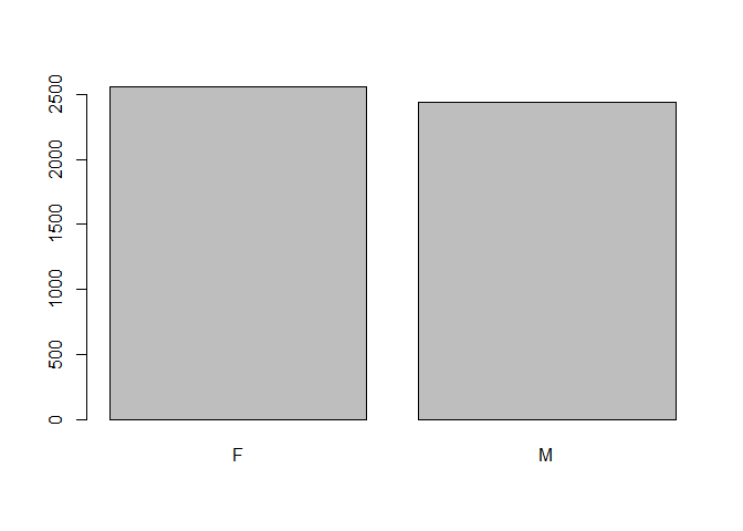
Plotting Factor Variables with Barplots
You can also wrap the plot() function around vector of factors to get a barplot. Barplots are used to get the counts of how many rows belong to each factor variable.
plot(data$gender)
Creating Pivot Tables
table(data$gender, data$virus)
##
##        N    Y
##   F 1127 1430
##   M 1315 1128
Numeric variables
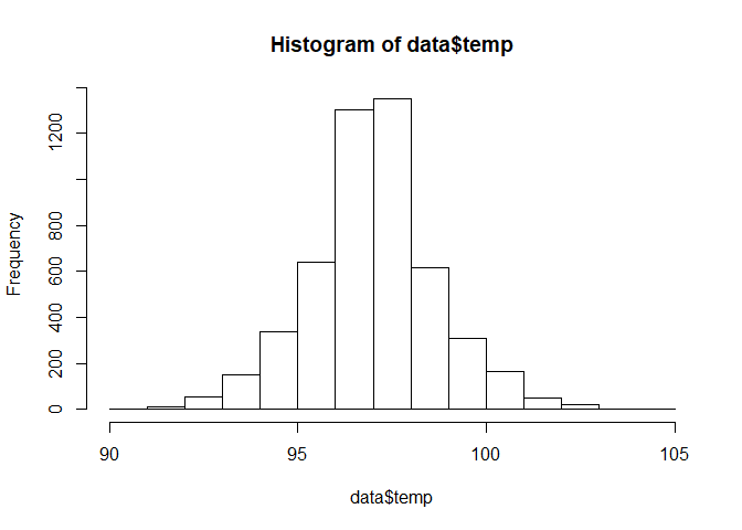
Numeric variables on the other hand are quite different. While we can still use the table() function to find the the distribution of the variables within a column, it is much better to use a histogram plot to find out the distribution While they looks similar, it is important to understand that Histograms are used to analyze the distribution of NUMERICAL data. Barplots are used to analyze the frequency of CATEGORICAL variables.
hist(data$temp)
We can also perform some handy statistical functions on numeric vectors.
# min(): returns the minimum value of a vector
min(data$temp)
## [1] 90
# max(): returns the maximum value of a vector
max(data$temp)
## [1] 105
# sd(): returns the standard distribution value of a vector
sd(data$temp)
## [1] 1.713411
# mean(): returns the mean of a vector()
mean(data$temp)
## [1] 97.4968
Fixing Data
We can keep ID as a categorical (factor) variable, since it is just a unique identifier for our rows and we can’t extract meaningful insights from it. AgeGroup how ever can be vague. It is displayed as integer, but we don’t know if a 0 indicate someone who is young or someone who is old. This could be a problem. Let’s tell R that this variable should be treated as a factor, and not an integer.
## Note: You turn ageGroup back into an integer using as.integer(data$ageGroup)
data$ageGroup <- as.factor(data$ageGroup)
Let’s use str() again to see if this variable has been transformed
str(data)
## 'data.frame':    5000 obs. of  6 variables:
##  $ id      : Factor w/ 5000 levels "1002","1003",..: 11 22 33 44 55 66 77 88 99 218 ...
##  $ gender  : Factor w/ 2 levels "F","M": 1 2 1 2 1 2 2 1 1 2 ...
##  $ ageGroup: Factor w/ 3 levels "0","1","2": 3 3 1 2 1 1 1 3 3 3 ...
##  $ pulse   : int  58 55 51 68 77 56 61 73 56 56 ...
##  $ temp    : int  97 98 97 98 98 97 97 98 96 98 ...
##  $ virus   : Factor w/ 2 levels "N","Y": 1 1 1 2 2 1 1 2 1 1 ...
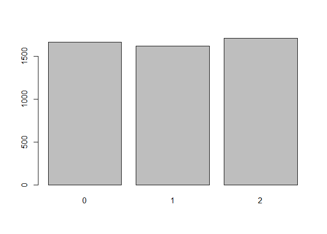
Now if we tried to plot the variable, we can see some instights. Using the plot() function on a categorical variable will give us a frequency barplot of groupings in the vector
plot(data$ageGroup)
Zoning In On Your Data
The DPLYR Select Command
You can use the select command to grab a subset of the columns in a dataframe.
data %>% select(id, gender, ageGroup)
##        id gender ageGroup
## 1     101      F        2
## 2     102      M        2
## 3     103      F        0
## 4     104      M        1
## 5     105      F        0
## 6     106      M        0
## 7     107      M        0
## 8     108      F        2
## 9     109      F        2
## 10    11F      M        2
## 11    11M      M        0
## 12    112      F        1
## 13    113      M        2
## 14    114      F        0
## 15    115      M        1
## 16    116      F        1
##  [ reached getOption("max.print") -- omitted 4984 rows ]
Unselecting columns
What if you wanted to select everything but a handful of columns? While there’s no Unselect() function, you can apply a minus sign to the columns within select() function, to grab everything except those columns specified.
data %>% select(-id,-ageGroup)
##      gender pulse temp virus
## 1         F    58   97     N
## 2         M    55   98     N
## 3         F    51   97     N
## 4         M    68   98     Y
## 5         F    77   98     Y
## 6         M    56   97     N
## 7         M    61   97     N
## 8         F    73   98     Y
## 9         F    56   96     N
## 10        M    56   98     N
## 11        M    67   97     N
## 12        F    71  100     Y
##  [ reached getOption("max.print") -- omitted 4988 rows ]
The DPLYR: Filter Command
Just as you can select columns, you can also select certain rows. You do this by FILTERing your data frame. Let’s say that we wanted to examine our female population in the dataset. The filter() function allows you to pass in a boolean statement. A boolean statement is a statement that can be evaluated as true or false. In this case, any rows that do not have the value of ‘F’ in there gender column will be evaluated as False, and therefore be filtered out.
# NOTE:  the single equal sign (=) is used as the assignment operator.
# Use the double equal sign (==) when using boolean statements.

data %>% filter(gender == "F")
##        id gender ageGroup pulse temp virus
## 1     101      F        2    58   97     N
## 2     103      F        0    51   97     N
## 3     105      F        0    77   98     Y
## 4     108      F        2    73   98     Y
## 5     109      F        2    56   96     N
## 6     112      F        1    71  100     Y
## 7     114      F        0    56   95     N
## 8     116      F        1    74  102     Y
##  [ reached getOption("max.print") -- omitted 2549 rows ]
Chaining Filters Together
You are also not limited to one filter, you can chain multiple conditional expression together using logical operators. If you are new to R, here is a link to R’s logical operators. {link}
# The & symbol is the 'AND' Operator
# This sentence read: Give me all the patients who are female AND who are of ageGroup 2 AND who have a virus.
# This means that all rows returned must have those conditions must be satisfied.
data %>% filter(gender == "F" & ageGroup == 2 & virus == "Y")
##       id gender ageGroup pulse temp virus
## 1    108      F        2    73   98     Y
## 2    118      F        2    70  100     Y
## 3    119      F        2    63   98     Y
## 4    12F      F        2    58   98     Y
## 5    132      F        2    90   98     Y
## 6    142      F        2    77   98     Y
## 7    149      F        2    75   98     Y
## 8    15F      F        2    76   99     Y
##  [ reached getOption("max.print") -- omitted 493 rows ]
Other Options To Filtering
Let’s say there were a group of subjects we wanted to examine in our datset that we couldn’t exactly filter using the columns. A case like this might occur when we might want to match observations to a specific set of values. Let’s grab the data for id 108, 15F, and 12F.
# The | symbol is the 'OR' Operator
# This reads as: Give me the patients who have an id of 108 OR 15F or 12F.
# For OR logical statements, only one of the those boolean expressions need to be true,
# and since you have three boolean expressions on a distinct factor variable, you get back three rows.

head(data %>% filter(id == "108" | id == "15F" | id == "12F" ))
##    id gender ageGroup pulse temp virus
## 1 108      F        2    73   98     Y
## 2 12F      F        2    58   98     Y
## 3 15F      F        2    76   99     Y
What’s %in% Here?
That wasn’t so bad for three observations, but what if there was more? It would be nice to store these id’s in some sort of data structure where they can be used again in the future. Let’s pass those Id’s to a vector and use the %in% keyword to extract those items from the list. The %in% keyword let’s us save unique values in a data structure so we can reuse them.
interesting_ids <- c('108','15F', '12F')


data %>% filter(id %in% interesting_ids)
##    id gender ageGroup pulse temp virus
## 1 108      F        2    73   98     Y
## 2 12F      F        2    58   98     Y
## 3 15F      F        2    76   99     Y
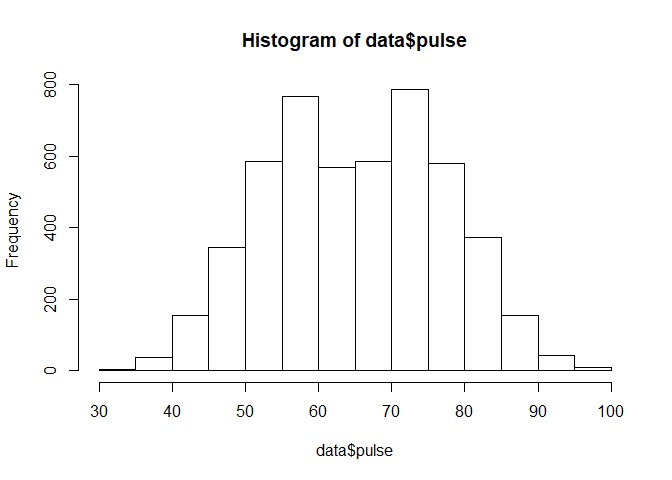
Creating New Variables From Old Ones
As you can see, the pulse variable has two humps, instead of your normal “bell” shaped distribution. Therefore, we can say that this variable is bimodal, depending on what kind of analysis you are trying to perform, bimodal distributions may pose a challenge. Can we transform this tricky numeric variables into a factor variable with a more uniform distribution?
hist(data$pulse)
Introducing Conditionals: IF-Else
If you already come from a programming background, then you will already be familiar with condtional statements. They work slightly different in R, but the syntax should feel similar.
# SYNTAX
# ifelse( BOOLEAN EXPRESSION, RESULT IS TRUE, RESULT IS FALSE)

age <- 21

buyBeer <- ifelse(age >= 21, "Yes, I am are old enough", "No too young :( ")

print("Can you buy beer?")
## [1] "Can you buy beer?"
print(buyBeer)
## [1] "Yes, I am are old enough"
Introducting MUTATE()
The majority of the time, the features we want in the data are not explictly contained in a column. Feature engineering is a huge topic in data science and one that cannot be covered in a single blog post. The main idea is that we can create and extract better variables from the ones that are already present in our dataset. One such case is creating categorical variables from numerical data. DPLYR’S MUTATE keyword, in combination with conditional statements, allows us to do this. In this example, we will be creating a new variable called ‘pulse_group’, which will be an evenly distributed categorical variable for the pulse variable.
# Syntax for MUTATE
# data frame %>% mutate(NEW VARIABLE = LOGIC FROM Old Variables)


data <- data %>% mutate(pulse_group = ifelse(pulse > 72, "High",
                                              ifelse(pulse > 58, "Medium",
                                                "Low")))


barplot(table(data$pulse_group))
The PitFalls of If-Else and A Case for Case Statements
You may have noticed the that tricky ifelse statement. If-Else statements are great for simple one-liners, but as you saw in the previouse example, they are not build to scale. A better alternative would be a case statement, which are handy way to define and scale conditional statements.
# ###############################################
# IFELSE ##
# ##############################################
# Syntax:
# ifelse( [condition 1], result 1 ,
# ifelse( [condition 2], result 2,
# ifelse(.......)))
# VS
# Case When ##
# ##############################################
# Syntax
# case_when(
# [condition 1] ~ result 1
# [condition 1] ~ result 2,
# ....
# [condition x] ~ result x
# #############################################
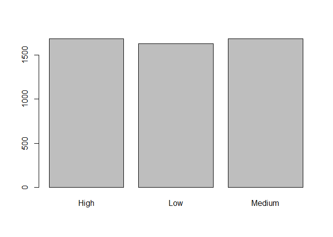
data <- data %>% mutate(pulse_group = case_when(
pulse > 72 ~ "High",
pulse > 58 ~ "Medium",
TRUE ~ "Low"))
table(data$pulse_group)
##
##   High    Low Medium
##   1686   1629   1685
barplot(table(data$pulse_group))

Putting It All Together
The beautiful thing abour DPLYR is that you can chain functions together usng the %>% operator, to create powerful, yet easy to read data frames. For example, let’s say we wanted to create a new dataframe with the following restrictions.
- Must be all men
- A new categorical variable, pulse_group, must be created from pulse using MUTATE()
- Select only the ID, pulse_group, and virus
new_data <- data %>% filter(gender == 'M') %>%
                    mutate(temp_group = case_when(
                                                temp > 99 ~ "High",
                                                temp > 95 ~ "Medium",
                                                TRUE ~ "Low")) %>%
                    select(id, pulse_group, virus )


head(new_data)
##    id pulse_group virus
## 1 102         Low     N
## 2 104      Medium     Y
## 3 106         Low     N
## 4 107      Medium     N
## 5 11F         Low     N
## 6 11M      Medium     N
Some new insights
With our new dataset, let’s explore how virus is distributed among the pulse grou variable.
table(new_data$pulse_group, new_data$virus)
##
##            N   Y
##   High    34 709
##   Low    841  39
##   Medium 440 380
Conclusion
If you been following along, you should have gained some familiarity with R’s DPLYR package. There’s alot more that we didn’t cover in this article.